Machine Learning Capabilities with Oracle Analytics Cloud

Machine Learning Capabilities with Oracle Analytics Cloud

The latest version of Oracle Data Visualization (v4.0) introduces a machine learning feature that lets users to build and make predictions using your existing data.

These models are classified like

        ·         Numeric Prediction (Numeric Prediction against new data)

        ·         Classification (Prediction against new data, Classification/labels are known)

        ·         Clustering (understand the structure of the data without a known classification Oracle DV offers several ML algorithms to support various versions (Numeric prediction. Multi Classification, two classification and clustering).

Typical Workflow to Analyse Data with Machine Learning in Oracle DV

        

     Train Numeric Prediction: Apply this model to you are data to predict a numeric value based on the known data values. Train numeric prediction node considers all input columns  in the data set, but built the model only using columns which it find to have a decisive influence on determining the target value.

Example: You might predict CPU performance.

We train binary classification using the train Numeric prediction step by step:

è Create or open data flow.

è Click on add step (+), then click on Train Binary Classification.

è In the select Train Numeric Prediction model script dialog, select script

1.       CART (Classification and Regression Tree) for model training: Uses decision tree to predict both discrete and continue values. It can be used when working with large data sets.

2.       Elastic net linear regression for model training: It is an advanced regression method. It does regularisation (adds additional information), variable section and linearly combines penalties lasso and ridge regression method. This is useful in cases with large number of attributes to avoid collinearity (multiple attributes being perfectly correlated) and over fitting.  

3.       Linear regression: It is a linear approach for modelling relationship between target variable and other attributes in the data set. This model can be used to predict numeric values when the attributes are not perfectly correlated.

4.       Random forest classification: It can ensemble learning method that constructs multiple decision trees and outputs the value that collectively represents all the decision trees. It can predict both numeric and categorical variables.

è Click on ok.

è Click on select column and select the data column to analyse.

è Click on save. And finally Run Data Flow.

Train Multi-Classifier Model: Apply this model to classify your data into three or more predefined categories.

Example: you may predict pic of fruits is apples, orange or banana

           We train binary classification using the train Multi classification step by step:

è Create or open data flow.

è Click on add step (+), then click on Train Binary Classification.

è In the select Train Multi-Classification model script dialog, select script

1.       CART (Classification and Regression Tree) for model training:  Uses decision tree to predict both discrete and continue values. It can be used when working with large datasets.

2.       Naive Bayes for classification: Is a probabilistic classification based on Bayes’ theorem with assumption that there is no dependent between features. It is used in when they are high number of input dimensions.

3.       Neural network for classification: Is an iterative classification algorithm that learns by comparing its classification results with the actual value and feedback it to the network to modify the algorithm for further iterations. This is used for text analysis.

4.       Random forest for model classification: Is ensemble learning method that constructs multiple decisions trees and outputs the values that collectively represents all the decision trees. It can be used to predict both numeric and categorical variables.

5.       SVM (support vector machine) for classification: It classifies vectors by mapping them in space and constructing hyper planes which can be used for classification. New records (scrolling data) are then mapped onto the space and are predicted belong to category based on which side on hyper planes they fall.

è Click on ok.

è Click on select column and select the data column to analyse.

è Click on save. And finally Run Data Flow.

Train Binary Classification: To predict attrition have two values yes/no.

Apply Binary classification model to classify your data into one of two predefined categories.

Example: you might predict whether product instance will pass or fail to quality control test.

We train binary classification using the train binary classification step by step:

è Create or open data flow.

è Click on add step (+), then click on Train Binary Classification.

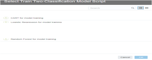
è In the select Train Two-classification model script dialog, select script

1.       CART (Classification and Regression Tree) for model training.

2.       Logistic regression algorithm.

3.       SVM (support vector machine) for classification.

4.       Naive Bayes for classification.

5.       Neural network for classification.

6.       Random forest for model classification.

è Click on ok.

è Click on select column and select the data column to analyse.

è Click on save. And finally Run Data Flow.

Train Clustering:  Apply this model to identifying the similar records assign them into one cluster.

             We train binary classification using the Train Clustering step by step:

è Create or open data flow.

è Click on add step (+), then click on Train Clustering.

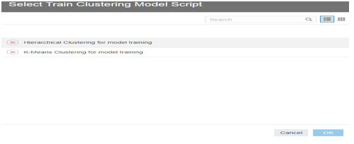
è In the select Train Clustering model script dialog, select script

1.       Hierarchical Clustering for Classification: It builds a hierarchy of clusters using either bottom-up of top-bottom. Hierarchical clustering is usually used when the data set is not big and number of clusters in not known beforehand.

2.       K-Means Clustering for Classification: It is iteratively partition records into k clusters in which each observation belongs the cluster with nearest means. It can be used for clustering metric columns and with a set expectations of number of clusters needed. it is known to work well with the large data sets. Results will also be different with each run unlike hierarchical clustering.

è Click on ok.

è Click on save. And finally Run Data Flow.

 After created model then we can viewed or accessed in Machine Learning Tab.

         To view more details about each model quality, like Accuracy, Confusion Matrix etc., inspect the model.

          In that we can see the quality tab for the model. You will found the model quality details like below:

Types Of Tables In Oracle Database

Types of Tables in Oracle Database

Creating a Table:

To create a table, you need to define three things:

• Name of the table.
• Columns in the table.
• Datatypes of those columns

The basic syntax for creating table is :

Create table <table_name> (

<column_name 1> <data_type>,

<column_name 2>  <data_type>,

<column_name 3> <data_type>,

….

)

In Oracle, there are different types of tables. Each type of table have it's own characteristics. 

Type of Tables:

           1.      Heap Organized Table.

           2.      Index Organized Table.

           3.      External Table.

           4.      Cluster Table.

           5.      Temporary Tables.

Heap Organized Table:

        The default type of table in Oracle is heap table. If you use ‘Create table’ clause normally, you create a standard database table. A heap Organized Table is a table which does not stores rows in a particular order. This means the database free to store rows wherever there is space. You can add “Organization heap” if you want to be explicit:

Example: Create table student (id int, name char (20), sub char (20), marks int);

(Or)

Create table student (id number(10), name varchar2(20), sub char (20), marks number(10)) Organization heap;

Advantages of Heap Organized table:
                 ·        Heap tables are Very fasted to insert data.
                  ·      The Heap Table does not have any non clustered index. Then the entire table will examined to find any row. This is applicable when the table is tiny. 

Disadvantage of Heap organized table:

                ·        The heap table will not applicable for large tables.
                 ·        When you want to access the data form large tables then it is very slow to access the data.

Index Organized Table:

         A row in an Index Organized Table (IOT) does not have a stable physical location. It keeps data in sorted order. Index Organized Table (IOT) have their primary key data and non-key columns data stored with in the same B-Tree structure. The data will stored in the primary key index.

         To Create Index Organized Table you need:

                

             ·        Specify the primary key using a column or table constrain.

             ·        Use the ORGANIZATION INDEX.

Example:

Create table student (id number(10), name varchar2(20), marks number(10), constrain pk_student primary key(id))

Advantages of Index Organized Table:

          ·        Index Organized Tables make accessing data via the primary key quicker as the key and the data reside in the same structure.
           ·        Since there is no need to read an index, the table data is read in a separate structure.
            ·        Less duplication of the key columns in an index and table mean low storage requirements

·        Increased performance: There is no need to access a row in the database from an index structure, so you can reduce the total number of operations needed to retrieve data.

·        Reduced table space: Because you do not need to link to a row in a table, there is no need to store the ROW ID in the index. The overall space required for the table is reduced.

·        Presorted data: The data in the leaf nodes is already sorted by the value of the primary key.

Disadvantages of Index Organized Table:

       ·        You must have a primary key on the table with a unique value.

       ·        You cannot have any other indexes on the data.

       ·        You cannot partition an index-organized table.

       ·        An index-organized table cannot be a part of a cluster.

       ·        The data in the row must be fairly small. Large amounts of data in the leaf nodes will require more to retrieve it.

External Table:

            External tables allow Oracle to query data that is stored outside the database in flat files. The ORACLE_LOADER driver can be used to access any data stored in any format that can be loaded by SQL*Loader. No DML can be performed on external tables but they can be used for query, join and sort operations. Views and synonyms can be created against external tables. They are useful in the ETL process of data warehouses since the data doesn't need to be staged and can be queried in parallel. They should not be used for frequently queried tables.

            You use external tables to read non-database files on the database server. For example, comma-separated values (CSV) files. To do this, you need to:

• Create a directory pointing to the location of the file on the server
• Use the organization external clause
• State the directory and name of the file you want to read

Creation of External Table:

            Create the external table using the CREATE TABLE..ORGANIZATION EXTERNAL syntax. This defines the metadata for the table describing how it should appear and how the data is loaded.

Example:

create or replace directory student_dir as '/myfile';

create table Student  (

Student_name varchar2(100)

) organization external (

default directory tmp

location ('student.csv')

);

Note: Live SQL doesn't support external tables. So these statements will fail!

When you query this table, it will read from the file:

/myfile/student.csv

This file must be accessible to the database server. You cannot use external tables to read files on your machine.

Advantages of External Tables:

            ·        External tables can be selected, sorted, filtered, joined, intersected, misused, unioned and so on using SQL, the language most familiar database to Oracle developers.
              ·         Loading a table from an external table is faster than SQL*Loader due to parallel query and DML.
                ·        External tables do not require any database space; only the space consumed by the flat-files on the file system.

Cluster Table:

            Use the CREATE CLUSTER statement to create a cluster. A cluster is a schema object that contains data from one or more tables, all of which have one or more columns in common. Oracle Database stores together all the rows from all the tables that share the same cluster key.

            After you create a cluster, you  can add tables to it. A cluster can contain a maximum of 32 tables. After you create a cluster and add tables to it, the cluster is transparent. You can access clustered tables with SQL statements just as you can access non clustered tables.

Creation of Cluster Table:

create cluster emp_cluster (

  emp_name varchar2(100)

);

Then place your tables in it using the cluster clause of create table:

create table emp_table (

  emp_name varchar2(100)

) cluster emp_cluster ( emp_name );

create table dept_table (

  dept    varchar2(20),

  emp_name varchar2(100)

) cluster emp_cluster ( emp_name );

Rows that have the same value for emp_name in emp_table and dept_table will be in the same place. This can make it faster to get a row for a given emp_name from both tables.

Temporary Tables:

           

           Temporary tables store session specific data. Only the session that adds the rows can see them. This can be handy to store working data.

     Oracle support two types of temporary tables:

·        Global Temporary Tables:

To create a global temporary table add the clause "global temporary" between create and table. For example:

Create global temporary table emp_table (emp_name varchar2(100))

The definition of the temporary table is permanent. All users of the database

can access it.But only your session can view rows you insert.

·        Private Temporary Tables:

These tables are only visible in your session. Other sessions can't see the table. To create one use "private temporary" between create and table. 

                   create private temporary table emp (emp_name varchar2(100));

    For both temporary table types, by default the rows disappear when you end your transaction. You can change this to when your session ends with the "on commit" clause.

   

    But either way, no one else can view the rows. Ensure you copy data you need to permanent tables before your session ends.